A Proportional-Integral-Derivative controller (PID) controller consists of a proportional unit (P), an integral unit (I) and a derivative unit (D). The PID controller is used with systems that has a desired linear response output with unchanging dynamic characteristics over time. The PID controller is a common feedback loop found mostly as a component of industrial control applications. The controller compares the collected data with a reference value and then uses this difference to calculate a new input value. The purpose of this new input value is to allow the system data to reach or stay at the reference value. The PID controller can adjust the input value based on the historical data and the occurrence rate of the difference to make the system more accurate and stable.
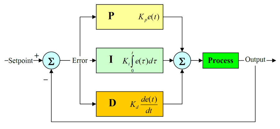
Through the Kp, Ki and Kd three parameter setting Due to its versatility and flexibility of use, it has serialized products and only three parameters (Kp, Ti, and Td) that can be manually and automatically adjusted based on the reference value and current output value. In many cases, not all three units are necessary, and one to two of them may be taken, but the proportional control unit (or the Kp value) is indispensable. In practice PID control doesn’t work well when controlling nonlinear, time-varying, coupled, and complex processes with a lot of variability in its parameters. Despite these drawbacks, simple PID controllers are sometimes the best controllers. Although many industrial processes are nonlinear or time-varying, by simplifying the process it can become a system where the basic linear and dynamic characteristics do not change over time so that it may be controlled via PID. That is, the PID parameters Kp, Ti and Td can be set in time according to the dynamic characteristics of the process. If the dynamic characteristics of the process change, for example, the dynamic characteristics of the system may change due to changes in the load and the PID parameters can be reset.
Theory
Open loop control system An open-loop control system means that the output (controlled amount) of the controlled object has no effect on the input of the controller. In such a control system, it does not rely on returning the controlled quantity back to form a closed loop. Even closed-loop feedback controllers must operate in an open-loop mode on occasion. A sensor may fail to generate the feedback signal or an operator may take over the feedback operation in order to manipulate the controller’s output manually. Operator intervention is generally required when a feedback controller proves unable to maintain stable closed-loop control. For example, a particularly aggressive pressure controller may overcompensate for a drop in line pressure. If the controller then overcompensates for its overcompensation, the pressure may end up lower than before, then higher, then even lower, then even higher, etc. The simplest way to terminate such unstable oscillations is to break the loop and regain control manually. There are also many applications where experienced operators can make manual corrections faster than a feedback controller can. Using their knowledge of the process’ past behavior, operators can manipulate the process inputs to achieve the desired output values later. A feedback controller, on the other hand, must wait until the effects of its latest efforts are measurable before it can decide on the next appropriate control action. Predictable processes with longtime constants or excessive dead time are particularly suited for open-loop manual control. Closed loop control system A closed-loop control system means that the output of the controlled object (the controlled variable) is sent back to the input of the controller, forming one or more closed loops. The closed-loop control system has positive feedback and negative feedback. If the feedback signal is opposite to the system setpoint signal, it is called negative feedback. If the polarity is the same, it is called positive feedback. Generally, the closed-loop control system uses negative feedback. , also known as a negative feedback control system. There are many examples of closed-loop control systems. For example, a person is a closed-loop control system with negative feedback. The eye is a sensor and acts as a feedback. The human body can make various corrective actions through constant correction. Without eyes, there is no feedback loop and it becomes an open-loop control system. In another example, when a genuine fully automatic washing machine has the ability to continuously check whether the laundry is washed and can automatically cut off the power after washing, it is a closed-loop control system. The step approaches are the output of the system when a step function is added to the system. The steady-state error refers to the difference between the expected output and the actual output of the system after the system response enters the steady state. The performance of the control system can be described in terms of stability, accuracy, and speed. Stability refers to the stability of the system. A system must be able to work properly. It must be stable first, and it should be convergent from the point of view of the step response. It refers to the accuracy and control accuracy of the control system. It is usually stable. Steady-state error describes the difference between the steady-state value of the system output and the expected value. Fast refers to the rapidity of the response of the control system and is usually described quantitatively by the rise time. As an example, let’s look at a space heater. Turning the heater off when the temperature sensor indicates that it is hotter than the set temperature and on when it is below the set temperature results in a system where the temperature “hunts” around the set temperature. Rather than simply switch a heater on and off, a feedback controller will adjust the output power to the heater (or other actuators) taking three factors into consideration (Kp, Ti, Td). Let’s look at how each of these factors affects the overall system. The Proportional Factor (Kp) Proportional control just means that the output power to the heater is proportional to the error. So bigger error values mean a larger difference between the actual temperature and the set temperature resulting in more power going to the heater. As the actual temperature gets close to the set temperature. Depending on the system, it will probably still overshoot, but not nearly as much as it does with a simple on/off control. It’s a bit like driving up to a stop sign: someone anticipating the stop sign will brake before reaching it rather than slamming on the brakes at the last possible moment.
u(t)=Ke(t)
The advantage of using proportional action is its simplicity. The pure P controller is easy to complement by a simple multiplication of the control error with the control error with the controller gain K. However, designing a P controller is always a trade-off. A high value of the proportional gain K result in fast setpoint tracking performance and fast disturbance rejection. The problem with the high value of K is that the measurement noise is amplified by K. This, again, might increase the risk of an unstable closed loop. If the system without integration is controlled, another undesirable property of pure P control is the closed loop steady-state error. The steady-state error depends on the value of K. The smaller the proportional gain K, the larger the steady- state error. The closed-loop steady-state error caused by setpoint input is obtained by calculating the error signal for the limit t
ess = lim e(t)
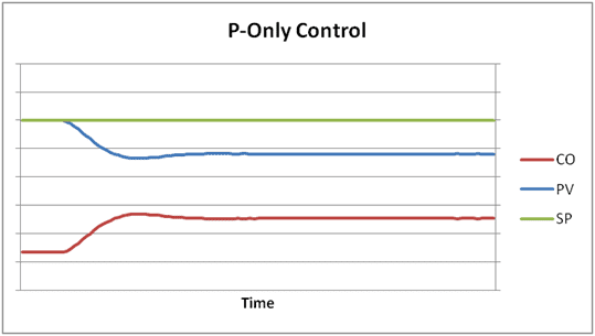
Under proportional-only control, the offset will remain until the operator manually changes the bias on the controller’s output to remove the offset. This is typically done by putting the controller in manual mode, changing its output manually until the error is zero, and then putting it back in automatic control. It is said that the operator manually “resets” the controller.
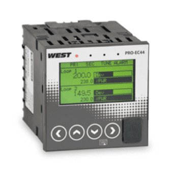
https://www.west-cs.com/products/l2/pid-temperature-controller
Proportional action can be used to improve the rise tie of the closed-loop response. If steady states error is not desired, it is required that the plant has an inherent integrating action. The inherently present integral action enables using pure P control without steady-state error. However, if the steady-state error is not a problem, then pure P control can also be used for plants without an integrating action. Even if pure P control can stabilize unstable plants, caution has to be exercised if the plant has a double integrator in its dynamics, Then, pure P control results in an unstable closed loop. When using the control structure with two degrees of freedom in the Laplace domain, the control error can be written as:
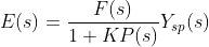
Thus, the final value theorem results in the steady-state error:

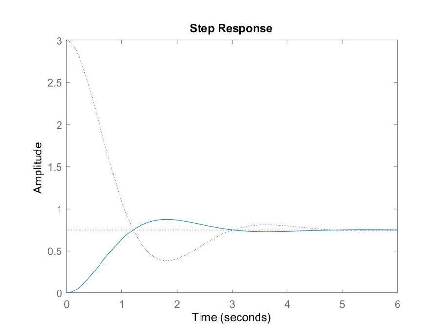
MATLAB The following code simulates the P-controlled second-order system of the example. The response of the control output “y“amd the control variable”u” (dotted line) to a unit step change at the input ysp for K=3 is plotted. P=tf(1,[1 2 1]);C=3;cl=feedback(series(C,P),1);step(c1); hold on;cl=feedback(C,P);step(cl,’:’);
PI control In addition to proportional action, integral action is used in the PI control. The purpose of an integral action is the elimination of the steady-state error. Therefore, using integral action leads to closed loop, whereas in the steady-state, the system output equals the set point. With integral action, the steady-state error can be eliminated, because even small errors lead to an increasing actuating signal. That is, the larger and the longer lasting the deviation of the system output to the set point, the more aggressive the control action. However, due to the required integration, the control signal might not build up fast enough to quickly compensate for step disturbances or step changes of the set point. Therefore, for the most practical applications, pure integral applications, pure integral control is not preferred. To increase the dynamics of pure I control, usually, the integral action is combined with proportional action, resulting in the well-known PI controller. The control Law of the PI controller is given by:

Transforming the control law into the Laplace domain results in the PI controller transfer function:
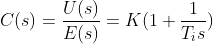
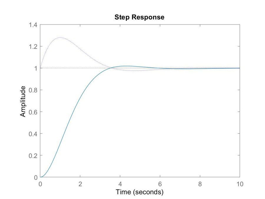
PI control combines the advantages of proportional action and integral action within one controller. It guarantees zero steady-state control errors, and the response to step changes of the set point or disturbances is faster compared to pure integral control. The advantage of PI control over pure I control in terms of fast response is illustrated. It should be mentioned that integral action is not necessarily required in the controller if the controller system already includes integral behavior inherently. Then, using pure proportional control does not result in a steady-state error. Matlab Executing the following code gives the response of the output “y” and the control signal “u” (dotted line) to a unit step change at the input ysp for K = 1 and Ti = 1.5: P=tf(1,[1 2 1]);C=tf([1.5 1],[1.5 0]);cl=feedback(series(C,P),1);step(cl); hold on;cl=feedback(C,P);step(cl,’:’);
PD control PD control allows for proportional action and derivative action in one controller. The control law and the transfer function of the ideal PD controller are given by:
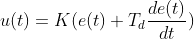

In the control law, the second term represents the rate of change of the error signal or the error function. Together with the first term, the PD controller gives a linear prediction of future errors. This predictive behavior makes the closed-loop response faster compared to pure proportional action or PI control. This, again, usually leads to improved stability and fewer oscillations of the closed-loop responses. However, the ideal PD controller is technically not realizable. Also, ideal PD control is not desired, because it results in the high-frequency gain, which amplifies measurement noise, and thus might lead to large control signals that can drive the actuator into saturation or might even cause damage. Therefore, in the presence of measurement noise, filtering of the derivative action in the high-frequency range is recommended. The filter is part of the PD controller, resulting in the following control law and transfer function:


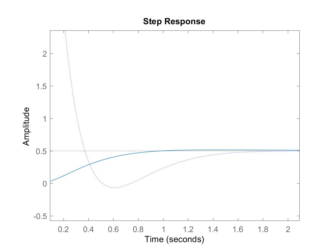
In order to influence the controller dynamics as little as possible, the chosen value of N has to be large enough. Simultaneously, the chosen N should not be too large, such that measurement noise is effectively suppressed. In the literature, different values for N are suggested. Values between 1 and 33 or 2 and 20 are mentioned. Choosing an optional value for N depends on the actual application, including the frequency range of the measurement noise. Note that in practical implementations derivative filtering might be automatically realized; for example, in the case in which the derivative term is digitally implemented by using the difference between two sampled values. However, inherent filtering might not be sufficient, and, therefore, additional low pass filtering can be required, according to equation 3.13 Matlab The above example can be reproduced by execution of the following code in Matlab. The response to unit step change at the input ysp of the output “y” and the control signal “u” (dotted line) for K = 1, Ti = 0.15, and Td = 1.5 are plotted. P=tf(1,[1 2 1]);C=tf([1.5 1],[0.15 1]);cl=feedback(series(C,P),1);step(cl); hold on;cl=feedback(C,P);step(cl,’:’);
Applications/Examples
Food Processing
- Regulating temperature
Controlling oil temperature in deep fryers can be hard to regulate. When the proper oil temperature is not being used, food can either get overcooked or under-cooked which can then lead to food waste. A precision PID controller can be used to set a proper temperature for cooking. This is very helpful in big food factories to make cooking processes efficient.
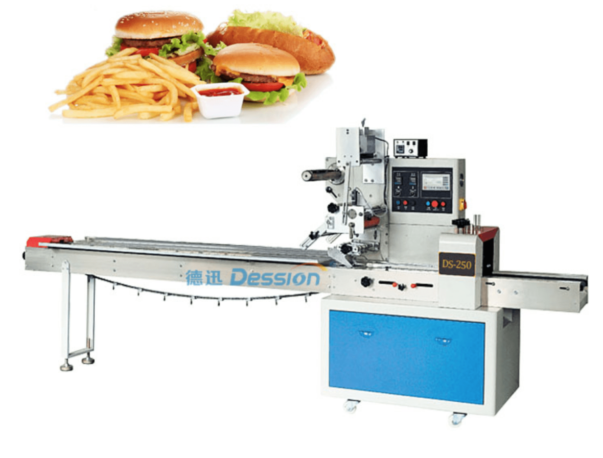
- Product Packaging
It is important that when products are being packaged that everything works simultaneously. The temperature, point of contact, and pressure when products are being sealed all have to be properly functioning and have to be repeatable for maximum efficiency.
Furnaces/Pottery
Kilns can be upgraded with PID controllers. Kilns with PID controllers can have ramp and soak functions. PID controllers with ramp and soak functions allow users to set the kiln to go up to a certain temperature and then let it soak or stay at that temperature for a certain period of time. Then the temperature can be set to change again after it has stayed at a certain temperature. The PID controller allows the user to not have to reset the kiln temperature multiple times and can help with reducing the number of times the kiln has to be checked while it is being used.
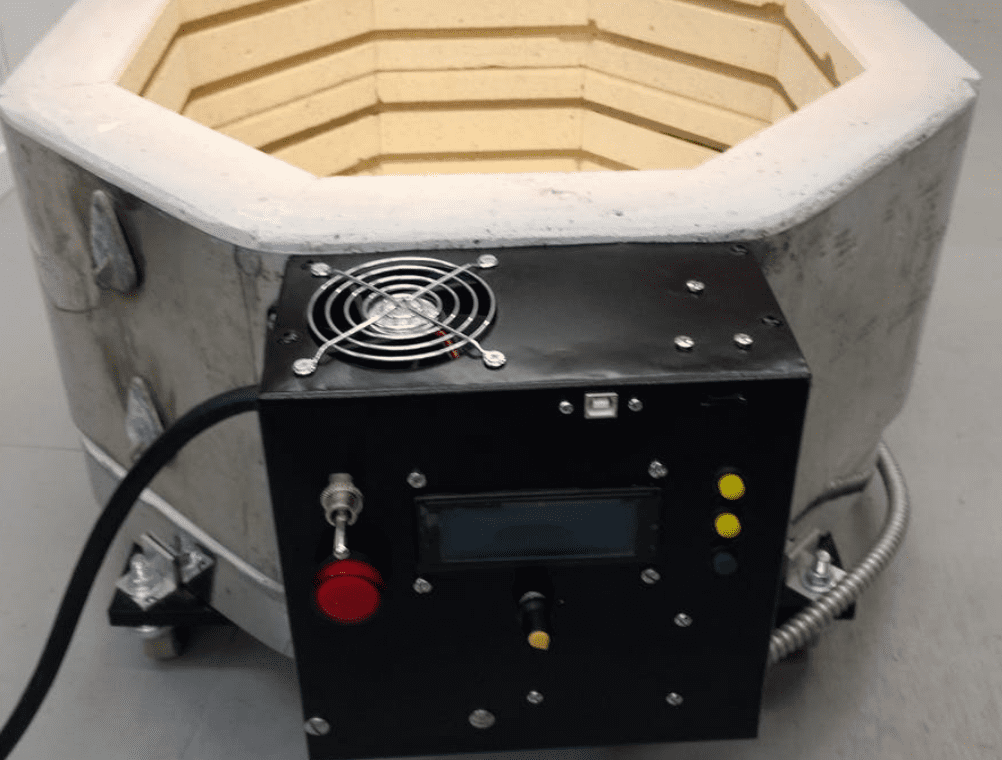
https://www.hackster.io/MrRoboto19/electric-kiln-controller-f5c633
Cleaning equipment
Single loop PID temperature controllers are normally used in medical cleaning equipment so that the machines work at the proper temperature for a certain amount of time so that medical supplies are appropriately sterilized. It works by using a temperature sensor that regulates the temperature inside the sterilizing tank and the PID temperature controllers determines whether or not the tank is running at the proper temperature.
DESIGN
PID control PID control combines the advantages of proportional action, integral action, and derivative action in one controller Proportional action gives the proportional response to the error signal, thus making the response fast. Integral action guarantees that steady-state control error disappears, and derivative action can contribute to additional closed-loop stability. The derivative term reduces oscillations, which usually allows for an additional increase of the proportional gain. This leads to a faster response of the closed loop in comparison to control without derivative action. However, a disadvantage of the derivative action is its noise amplifying character. Therefore, if derivative action is applied in the presence of excessive measurement noise, it should be considered to be filtering the error signal. Non-interacting Form The non-interacting form of the PID controller is characterized by a parallel structure, and it is also called the standard form. The advantage of the non-interacting form is that proportional, integral, and derivative action can be independently influenced by the controller parameters. The control law and the controller transfer function of the ideal PID controller in the non-interaction form are given by:


In real applications the derivative tern cannot be implemented as an ideal derivative. Therefore, the controller equation is subsequently amended with a first-order lag, resulting in the control law and transfer function of the real PID controller:


In contrast to filtering solely the derivative part, low pass fuktering can be applied alternatively to all controller terms. This, the ideal controller transfer function is additionally filtered with Gf(s)

For most applications, the filter Gf(s) is a one-order low-pass filter or a second-order low-pass filter. It is important to notice that PID controller design is usually done without considering a derivative filter. Thus, applying a derivative filter after the controller design results in additional errors, which might decrease the closed-loop control performance. In this situation, it is important to choose Ti carefully. When using the PID controller in the non-interacting form according to equation 3.17 the standard feedback control loop results as shown in Figure 3.5
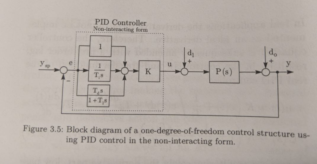
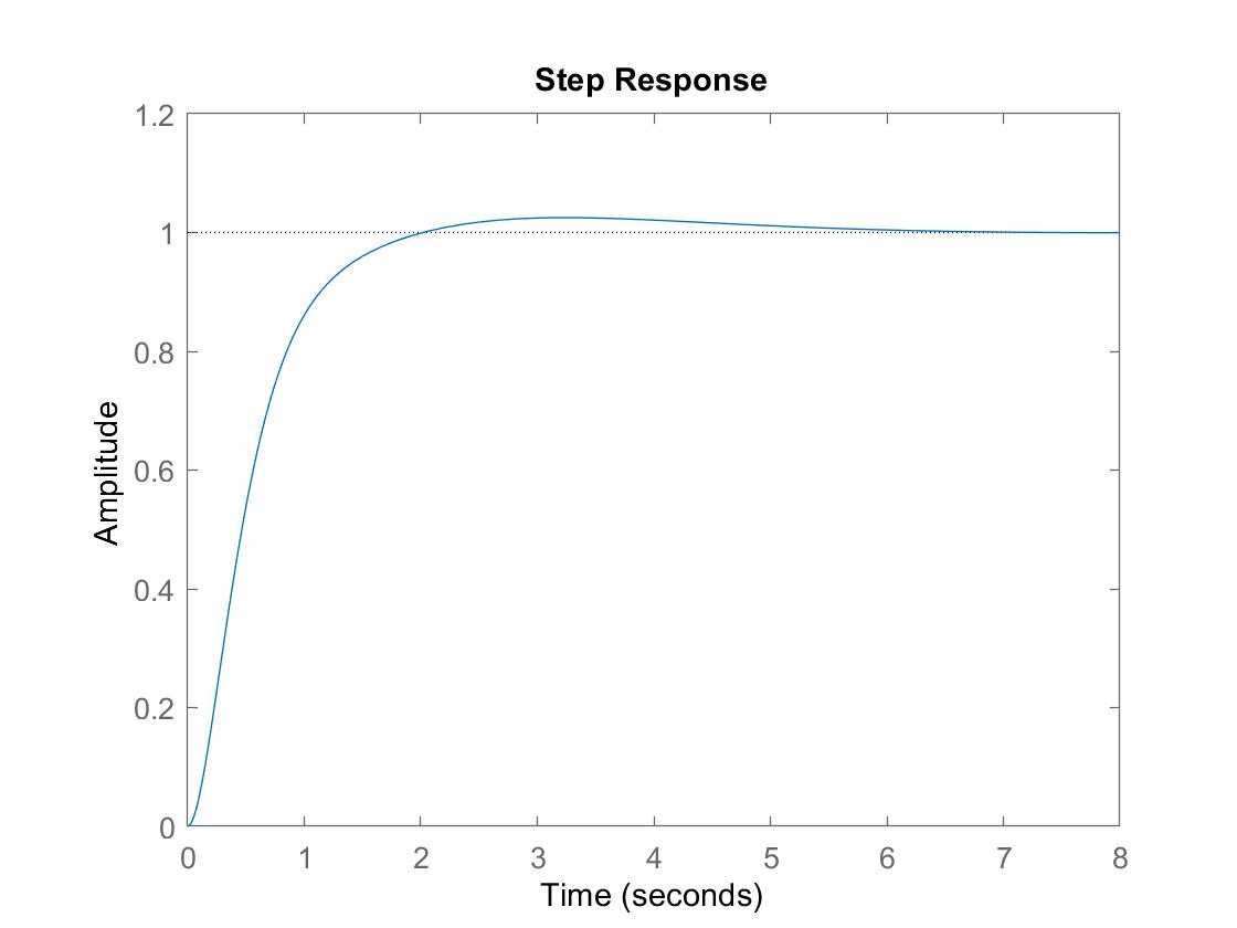
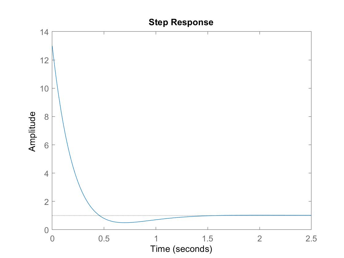
K, Ti, and Td, and can be adjusted independently and do not influence each other, which explains the name “non-interacting”. It is also very useful that with the non-interacting from complex zeros are possible, which is helpful when controlling oscillatory system. However, implementing the non-interacting form, for example in analog circuitry, requires more electronic components in comparison to realizing the interacting form.(The interacting form is discussed after the following example.) Matlab The following Matlab example gives the response of the PID-controlled closed-loop to a unit step change at the input. The parameters of the PID controller are set to K = 3, Ti = 1.5, and Td = 0.5. Executing the example in Matlab gives the output “y” and the control signal “u“. P=tf(1,[1 2 1]);K=3; Ti=1.5; Td=0.5;C=K*(1+tf(1,[Ti 0])+tf([Td 0], [0.15 1]));cl=feedback(series(C,P),1);figure;step(cl);cl=feedback(C,P);figure;step(cl);
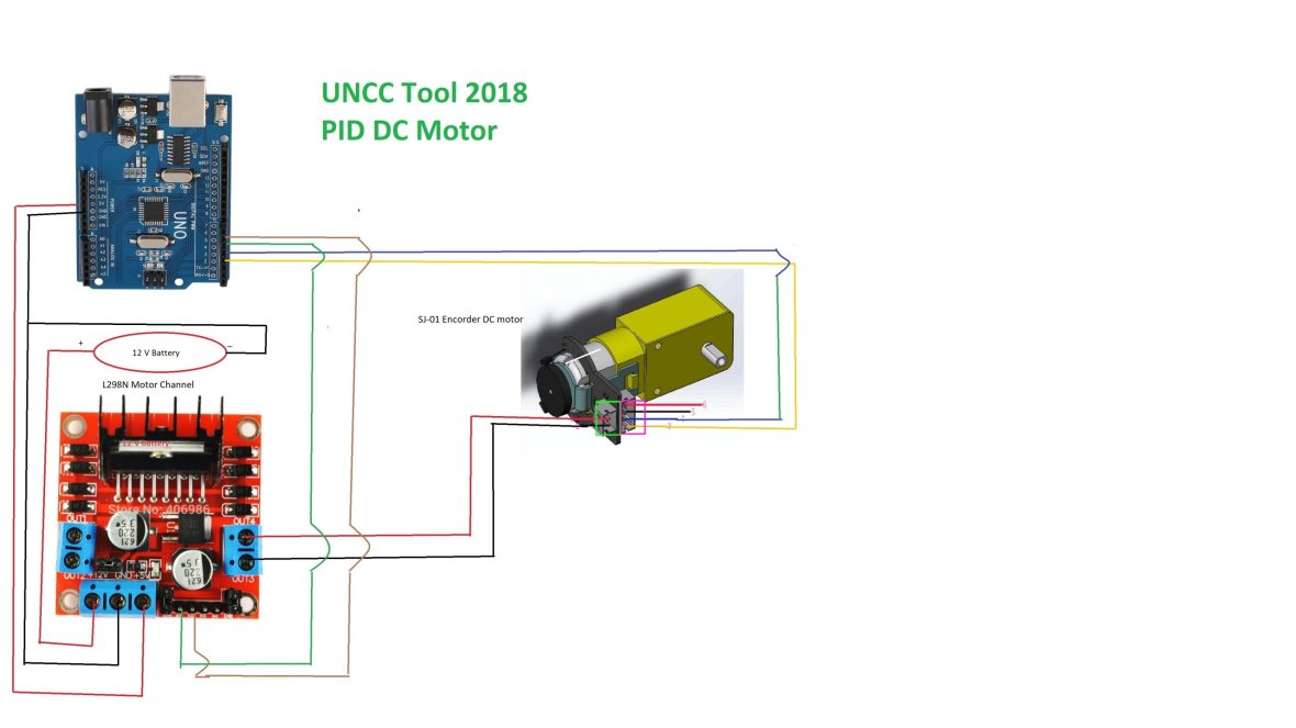
PID DC motor hardware demo
References
- Graf, Jens: “PID Control Fundamentals“, Columbia, SC. Accessed February 10, 2018.
- Smuts, Jacques F. “Process Control Consultant.” Control Notes. Accessed March 7, 2011. http://blog.opticontrols.com.
- Shelby, Nicole. “Make Action”. Edited by Roger Stewart. First Edition, January 2, 2018.
- Araki, M. and Taguchi, H.:Two-Degree-of-Freedom PID Controllers, International Journal of Control, Automation, and Systems Vol. 1, No. 4, 2003.
- Eshbach, O. W. and Kutz, M.: Feedback Systems: An Introduction for Scientists and Engineers, Princeton University Press, 2008.
- Ogata, K.: Modern Control Engineering (5th Edition), Prentice Hall 2009.
- VanDoren, Vance, Ph.D. “Open- vs. Closed-loop Control.” Next-generation Control Engineer Advice | Control Engineering. Accessed August 28, 2014. https://www.controleng.com/single-article/open-vs-closed-loop-control/d62442ec45d64b0e41b012e849b397a8.html.